Laje Vigada -Dimensionamento de armadura com Python

Exemplo de cálculo

Luis Moura / 2018-11-13

Introdução: Este texto, foi originalmente composto no Jupyter Notebook (Pérez and Granger 2007), usando a linguagem informática Python (Rossum and Drake 2001), sendo depois convertido para Rmarkdown (Allaire et al. 2016). Deixei visível todo o código informático que utilizei, de modo a que os resultados possam ser repetidos por outra pessoa ou simplesmente como referência para mim próprio.

Neste texto, pretendo com a ajuda da linguagem informática,¹ obter o dimensionamento da armadura para uma laje.

Condições existentes: O painel de lajes vigadas, representado na figura em baixo, apresenta uma espessura igual a 0.15 m e encontra-se submetido às seguintes acções:

peso próprio;
revestimento: \(1.5 kN/m^{2}\);
sobrecarga de utilização: \(4.0 kN/m^{2}\);

Objectivo: Dimensionar e pormenorize as armaduras das lajes do piso recorrendo ao método das bandas. Adoptar para materiais o betão C25/30 e aço A400NR.

Condições Iniciais

Livrarias necessárias

Introduzir as livrarias de Python (Rossum and Drake 2001), necessárias para este trabalho, que são Sympy (Meurer et al. 2017), AnaStruct (Vink, n.d.), Numpy (Travis E 2006) e Matplotlib.

%matplotlib inline
from anastruct.fem.system import SystemElements
import matplotlib.pyplot as plt
from sympy import*
init_printing(use_latex="mathjax")
x,y=var("x y",real=True)
import numpy as np
%load_ext tikzmagic

Gerar imagem da laje com LaTex

A imagem é criada usando os programas Tikz (Tantau 2013) e Stanli (Hackl 2016) para Latex (Donald E. Knuth, n.d.).

%%tikz --scale 1 --size 1000,500 -f png -p stanli --save=images/estrutura_2.png
\begin{tikzpicture}
\begin{scope}[shift={(1.5,3)}]
\scaling{1};%
\draw [help lines,step =.5] ( 0 , 0) grid (12 ,10);
\node[align=left] at (0,12.5) {Laje Vigada\\ Painel de Lajes Vigadas};
%draw the slab  
\point{a}{0}{0};
\point{b}{0}{5};
\point{c}{0}{10};
\point{d}{6}{10};
\point{e}{12}{10};
\point{f}{12}{5};
\point{g}{12}{0}
\point{h}{6}{0}
\point{i}{6}{5}
%Slab beams:    
\beam{1}{a}{b}[0][1];
\beam{1}{b}{c}[1][1];
\beam{1}{c}{d}[2][3];
\beam{1}{d}{e}[][];
\beam{1}{e}{f};
\beam{1}{f}{g};
\beam{1}{g}{h};
\beam{1}{h}{a}
\beam{1}{h}{i};
\beam{1}{i}{h};     
\beam{1}{i}{d};
\beam{1}{d}{i};
\beam{1}{b}{i}
\beam{1}{i}{b}
\beam{1}{i}{f}
\beam{1}{f}{i}
% Numbering beams   
\notation{1}{a}{A}[below left];
\notation{1}{b}{B}[below left];
\notation{1}{c}{C}[above left];
\notation{1}{d}{D}[above];
\notation{1}{e}{E}[above right];
\notation{1}{f}{F}[right];
\notation{1}{g}{G}[below right];
\notation{1}{h}{H}[below];
\notation{1}{i}{I};
%slab dimensions    
\dimensioning{2}{a}{b}{-1}[$5,0$];
\dimensioning{2}{b}{c}{-1}[$5,0$];
\dimensioning{1}{c}{d}{11}[$6,0$];
\dimensioning{1}{d}{e}{11}[$6,0$]
%points for the diagram
\point{A}{0}{-2};
\point{B}{6}{-2};
\point{C}{12}{-2};
\point{D}{14}{0};
\point{E}{14}{5};
\point{F}{14}{10}
\point{G}{14}{2.5}; %middle beam point
\point{H}{14}{7.5}; %middle beam point
%Diagram - Beams
\beam{2}{A}{B};
\beam{2}{B}{C};
\beam{2}{D}{E};
\beam{2}{E}{F}
%Supports for the diagram:
\support{1}{A};
\support{1}{B};
\support{1}{C};
\support{2}{D}[90];
\support{1}{E}[90];
\support{1}{F}[90];
%loads
\lineload{1}{A}{C}[0.5][0.5][.05];
\lineload{1}{D}{F}[0.5][0.5][.1];
%Moment Diagram 
\internalforces {A}{B}{0}{-.5}[-.5][ blue!40 ];
\internalforces {B}{C}{-.5}{0}[-.5][ blue!40 ];
\internalforces {D}{G}{0}{.5}[-.5][ blue!40 ];
\internalforces {G}{E}{.5}{-.5}[.5][ blue!40 ];
\internalforces {E}{H}{-0.5}{.5}[-.5][ blue!40 ];
\internalforces {H}{F}{.5}{0}[.5][ blue!40 ];
\end{scope}    
\end{tikzpicture}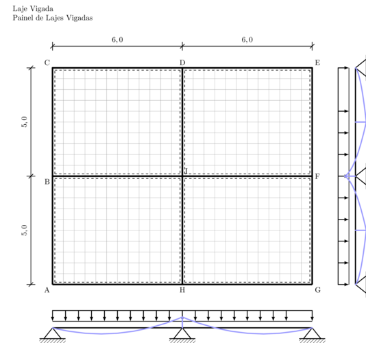

Condições Iniciais - Imagem gerada a partir de Tikz

Cálculo das Ações

Peso Próprio: pp \(= \gamma _ { \text { betao } } \times h = 25 \times 0.15 = 3.8 \mathrm { kN } / \mathrm { m } ^ { 2 }\)
Revestimentos: \(r e v = 1.5 \mathrm { kN } / \mathrm { m } ^ { 2 }\)
Sobrecarga: \(\mathrm { SC } = 4.0 \mathrm { kN } / \mathrm { m } ^ { 2 }\)

\[p _ { \mathrm { sd } } = 1.5 \mathrm { cp } + 1.5 \mathrm { sc } = 1.5 \times ( 3.8 + 1.5 + 4.0 ) = 13.9 \mathrm { kN } \mathrm { m } ^ { 2 }\]

Modelo de Cálculo

\(\frac { L _ { \text { maior } } } { L _ { \text { menor } } } = \frac { 6 } { 5 } = 1.2 < 2 \Rightarrow \text { Laje armada nas duas direcções }\)

%%tikz --scale 1 --size 750,600 -f png -p stanli --save=images/panel.png
\begin{tikzpicture}
\begin{scope}[shift={(1.5,9)}]
\scaling{1};%
\node[align=left] at (2,7) {Painel - Laje Vigada};

%Grid
\draw [help lines,step =.5] ( 0 , 0) grid (6 ,5);
%draw the slab  
\point{a}{0}{0};
\point{b}{0}{5};
\point{c}{6}{5};
\point{d}{6}{0};
%Slab beams:    
\beam{1}{a}{b};
\beam{2}{b}{c};
\beam{2}{c}{d};
\beam{1}{d}{a};
% Numbering beams   
\notation{1}{a}{A}[below left];
\notation{1}{b}{B}[above left];
\notation{1}{c}{I}[above right];
\notation{1}{d}{H}[below right];
%slab dimensions    
\dimensioning{2}{a}{b}{-1}[$5,0$];
\dimensioning{1}{b}{c}{6}[$6,0$];
%Draw the beam
\point{e}{0}{-3}
\point{f}{6}{-3};
\point{g}{0}{-4.5}
\point{h}{6}{-4.5}
% Draw Beam
\beam{2}{e}{f};
%Supports for the beam:
\support{1}{e};
\support{3}{f}[90];
%loads
\lineload{1}{e}{f}[0.5][0.5][.05];
\load{1}{e}[270][1][1];
\load{1}{f}[270][1][1];
%notations:
\notation{1}{g}{$ 3  \frac{pL}{8} $}[right];  
\notation{1}{h}{$ 5  \frac{pL}{8} $}[right]; 
%Draw the V points 
\point{i}{0}{-6}
\point{j}{6}{-6};
% Draw Beam V
\beam{2}{i}{j};
%Draw the V points 
\point{i}{0}{-6}
\point{j}{6}{-6};
% Draw Beam V
\beam{2}{i}{j};
% V Diagram 
\internalforces {i}{j}{-0.5}{0.8}[0][ black!90 ];
% Note  
\notation{1}{i}{DEV}[above left=3mm];
\notation{1}{i}{+}[above right];
\notation{1}{j}{--}[below left=3mm];
%Draw the M points 
\point{k}{0}{-8};
\point{l}{6}{-8};
\point{m}{2.5}{-8};
% Draw Beam V
\beam{2}{k}{l};
% V Diagram 
\internalforces {k}{l}{0}{-.5}[-.9][ black!90];
% Note  
\notation{1}{k}{DMF}[above left=3mm];
\notation{1}{m}{+}[below=1.5mm];
\notation{1}{l}{--}[above left];
\end{scope}   
\end{tikzpicture}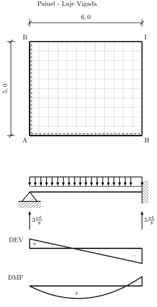

Cálculo dos Esforços - Direcção X

# Esforços na Direcção X
ss = SystemElements(load_factor=1 )
ss.add_truss_element(location=[[0, 0], [6, 0]])
ss.add_support_hinged(node_id=1)
ss.add_support_fixed(node_id=2)
Q=0.3*13.9 
ss.q_load(element_id=1, q=-Q)
ss.solve()
# get a visual of the element ID's and the node ID's
ss.show_structure(scale=0.6, figsize=(12,4))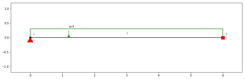

Diagrama do Esforço Transverso para a direcção x

\[V_{x=0-5.99}=9.38-4.2x\] \[V_{x=6}=9.38-4.2x+15.04\]

ss.show_shear_force(scale=0.6, figsize=(12,4))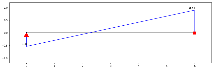

Diagrama de Momento Flector para a direcção X

Vx=-9.45+4.2*x
zero_a=solve(Eq(Vx,0),x)
zero=np.max(zero_a)
Mx=integrate(Vx)
print(f"Momento positivo máximo ocorre a {zero:.3} metros e é de {-Mx.subs(x,zero):.3} kNm/m."),
print(f"Momento negativo máximo ocorre aos 6 metros e é de {Mx.subs(x,6):.3} kNm/m.")
plot(Mx,(x,0,6), title=("DMF - Direcção X"));

Momento positivo máximo ocorre a 2.25 metros e é de 10.6 kNm/m.
Momento negativo máximo ocorre aos 6 metros e é de 18.9 kNm/m.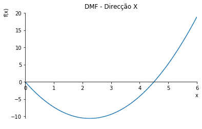

ss.show_bending_moment(scale=0.6, figsize=(12,4))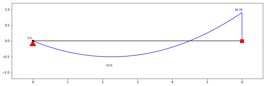

Cálculo dos Esforços - Direcção Y

# Esforços na Direcção Y
ss = SystemElements(load_factor=1 )
ss.add_truss_element(location=[[0, 0], [5, 0]])
ss.add_support_hinged(node_id=1)
ss.add_support_fixed(node_id=2)
Q=0.7*13.9 
ss.q_load(element_id=1, q=-Q)
ss.solve()
# get a visual of the element ID's and the node ID's
ss.show_structure(scale=0.6, figsize=(12,4))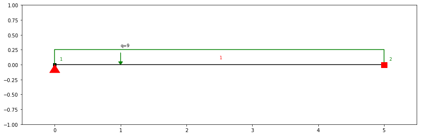

Diagrama do Esforço Transverso para a direcção Y

\[V_{x=0-5.99}=18.24-9.73x\] \[V_{x=6}=18.24-9.73.2x+30.41\]

ss.show_shear_force(scale=0.6, figsize=(12,4))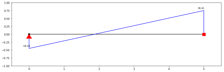

Diagrama de Momento Flector para a direcção Y

Vy=-18.24+9.73*x
zero_b=solve(Eq(Vy,0),x)
zero=np.max(zero_b)
My=integrate(Vy)
print(f"Momento positivo máximo ocorre a {zero:.3} metros e é de {-My.subs(x,zero):.3} kNm/m."),
print(f"Momento negativo máximo ocorre aos 6 metros e é de {My.subs(x,5):.3} kNm/m.")
c = Circle(Point(1.87,-17.1), 1)
plot(My, (x,0,5), title=("DMF - Direcção Y"), ylabel=("kNm/m"))

Momento positivo máximo ocorre a 1.87 metros e é de 17.1 kNm/m.
Momento negativo máximo ocorre aos 6 metros e é de 30.4 kNm/m.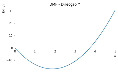

ss.show_bending_moment(scale=0.6, figsize=(12,4))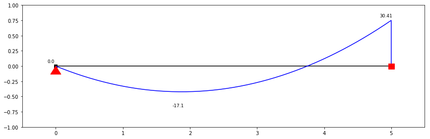

Tabela Resultados iniciais

\(M_{sd} ~ [kNm/m]\) - Momento Máximo Positivo e negativo em ambas as direcções

import pandas as pd
MX=[-Mx.subs(x,zero), -Mx.subs(x,6)]
MY=[-My.subs(x,zero), -My.subs(x,5)]
data = {'M (max) X-X' : pd.Series(MX), 
        'M (max) Y-Y' : pd.Series(MY)}
tabela = pd.DataFrame(data)
print(tabela)

         M (max) X-X        M (max) Y-Y
0   10.3353301736822   17.0964850976362
1  -18.9000000000000  -30.4250000000000

\(\mu\), Momento Reduzido

fcd=16.67
d=0.12
b=1
uxp=[N(-Mx.subs(x,zero)/(fcd*1000*d**2*b),3)]
uxn=[N(Mx.subs(x,6)/(fcd*1000*d**2*b),3)]
uyp=[N(-My.subs(x,zero)/(fcd*1000*d**2*b),3)]
uyn=[N(My.subs(x,5)/(fcd*1000*d**2*b),3)]
resultados=[uxp, uxn, uyp, uyn]
momentos=["Moment Max positivo,X-X",
          "Moment Max negativo,X-X",
         "Moment Max positivo,Y-Y",
         "Moment Max negativo,Y-Y"]
data_a = {'Descricao' : pd.Series(momentos), 
        'Momento Reduzido' : pd.Series(resultados)}
tabela_a = pd.DataFrame(data_a)
tabela_momento_reduzido=pd.DataFrame(tabela_a)
print(tabela_momento_reduzido)

                 Descricao Momento Reduzido
0  Moment Max positivo,X-X         [0.0431]
1  Moment Max negativo,X-X         [0.0787]
2  Moment Max positivo,Y-Y         [0.0712]
3  Moment Max negativo,Y-Y          [0.127]

\(\omega\)

wxp=[1-sqrt(1-2*N(-Mx.subs(x,zero)/(fcd*1000*d**2*b),3))]
wxn=[1-sqrt(1-2*N(Mx.subs(x,6)/(fcd*1000*d**2*b),3))]
wyp=[1-sqrt(1-2*N(-My.subs(x,zero)/(fcd*1000*d**2*b),3))]
wyn=[1-sqrt(1-2*N(My.subs(x,5)/(fcd*1000*d**2*b),3))]
resultados_omega=[wxp, wxn, wyp, wyn]
omega=["Omega positivo,X-X",
          "Omega negativo,X-X",
         "Omega positivo,Y-Y",
         "Omega negativo,Y-Y"]
data_b = {'Descricao' : pd.Series(omega), 
        'Valor de Omega' : pd.Series(resultados_omega)}
tabela_b = pd.DataFrame(data_b)
tabela_omega=pd.DataFrame(tabela_b)
print(tabela_omega)

            Descricao Valor de Omega
0  Omega positivo,X-X       [0.0439]
1  Omega negativo,X-X       [0.0822]
2  Omega positivo,Y-Y       [0.0740]
3  Omega negativo,Y-Y        [0.136]

Área de armadura, \(A_{s}\)


fsyd=348
Wxp=1-sqrt(1-2*N(-Mx.subs(x,zero)/(fcd*1000*d**2*b),3))
Wxn=1-sqrt(1-2*N(Mx.subs(x,6)/(fcd*1000*d**2*b),3))
Wyp=1-sqrt(1-2*N(-My.subs(x,zero)/(fcd*1000*d**2*b),3))
Wyn=1-sqrt(1-2*N(My.subs(x,5)/(fcd*1000*d**2*b),3))
As_x_p= [(Wxp*b*d*(fcd/fsyd)*10**4).n(3)]
As_x_n= [(Wxn*b*d*(fcd/fsyd)*10**4).n(3)]
As_y_p= [(Wyp*b*d*(fcd/fsyd)*10**4).n(3)]
As_y_n= [(Wyn*b*d*(fcd/fsyd)*10**4).n(3)]
resultados_As=[As_x_p, As_x_n, As_y_p, As_y_n]
As=["As,x+",
          "As,x-",
         "As,y+",
         "As,y-"]
data_c = {'Descricao' : pd.Series(As), 
        'Área de Armadura (cm2/m)' : pd.Series(resultados_As)}
tabela_c = pd.DataFrame(data_c)
tabela_As=pd.DataFrame(tabela_c)
print(tabela_As)

  Descricao Área de Armadura (cm2/m)
0     As,x+                   [2.53]
1     As,x-                   [4.72]
2     As,y+                   [4.25]
3     As,y-                   [7.82]

Armadura Miníma

\[A _ { s , m i n } = 0.26 \frac { f _ { c t m } } { f _ { y k } } b _ { t } \cdot d = 0.26 \frac { 2.6 } { 400 } \times 0.12 \times 10 ^ { 4 } = 2.03 cm ^ { 2 } /m\]

Esta armadura deve ser colocada em todas as zonas (e direcções) onde a laje possa estar traccionada.

Armaduras de distribuição

Armadura inferior: não é necessária
Armadura Superior: \(\mathrm { A } _ { \mathrm { s } , \mathrm { d } } = 0.20 \times 7.96 = 1.59 \mathrm { cm } ^ { 2 } / \mathrm { m }\) (direcção Y)
Armadura Superior: \(A _ { s , d } ^ { - } = 0.20 \times 4.81 = 0.9 \mathrm { cm } ^ { 2 } / \mathrm { m }\) (Direcção X)

Bibliografia

Allaire, JJ, Joe Cheng, Yihui Xie, Jonathan McPherson, Winston Chang, Jeff Allen, Hadley Wickham, Aron Atkins, and Rob Hyndman. 2016. Rmarkdown: Dynamic Documents for R. http://CRAN.R-project.org/package=rmarkdown.

Donald E. Knuth, Leslie Lamport. n.d. “LaTeX - a Document Preparation System.” LaTeX3 Project; https://www.latex-project.org/.

Hackl, Jürgen. 2016. “CTAN: /Tex-Archive/Graphics/Pgf/Contrib/Stanli.” https://ctan.org/tex-archive/graphics/pgf/contrib/stanli?lang=en.

Meurer, Aaron, Christopher P. Smith, Mateusz Paprocki, Ondřej Čertík, Sergey B. Kirpichev, Matthew Rocklin, AMiT Kumar, et al. 2017. “SymPy: Symbolic Computing in Python.” PeerJ Computer Science 3 (January): e103. doi:10.7717/peerj-cs.103.

Pérez, Fernando, and Brian E. Granger. 2007. “IPython: A System for Interactive Scientific Computing.” Computing in Science and Engineering 9 (3). IEEE Computer Society: 21–29. doi:10.1109/MCSE.2007.53.

Rossum, G. Van, and F.L. Drake. 2001. “Python Reference Manual.” Virginia, USA: PythonLabs. http://www.python.org.

Tantau, Till. 2013. The Tikz and Pgf Packages: Manual for Version 3.0.0. http://sourceforge.net/projects/pgf/.

Travis E, Oliphant. 2006. “A Guide to Numpy.” http://www.scipy.org/.

Vink, Ritchie. n.d. “Welcome to anaStruct’s Documentation! — AnaStruct 1.b3 Documentation.” https://anastruct.readthedocs.io/en/latest/index.html.

Fernando Pérez, Brian E. Granger, IPython: A System for Interactive Scientific Computing, Computing in Science and Engineering, vol. 9, no. 3, pp. 21-29, May/June 2007, doi:10.1109/MCSE.2007.53. URL: https://ipython.org ↩